Nearest Neighbor Density Estimation
Given a set of $d$ dimensional real-valued observations $X = {x_1, x_2, …, x_N}$, the $k$-Nearest Neighbor Density estimate $\hat{f}(x)$ for a given observation $x$ is given by the fraction of points in the sample within a sphere of radius $R_k$. We choose the radius to be the distance from $x$ to its $k$-th nearest neighbor. Finally, the ratio is scaled by the volume of the $d$-dimensional sphere, $V_{d, k}$ with radius $R_k$ so we have:
\(\hat{f}(x) = \frac{k}{N} \cdot \frac{1}{V_{d,k}}\),
where $V_{d, k} = \frac{\pi^{d/2}}{\Gamma(d/2 + 1)}R_k$.
Compared to KDE, this estimator has the advantage of being quick to compute for large datasests with high dimensionality using a KD-Tree. Variance in this estimator is independent of the dimensionality of the dataset (unlike with KDE) since the number of observations considered depends only on $k$. In a KDE, the bandwith does not directly determine the number of points considered in the estimate and the dimensionality of the data can have an influence. This comes with some caveats such as a heavy tail, see this and this for detailed descriptions.
Here is some code to play with the estimator:
import numpy as np
from scipy.special import gamma
from sklearn.neighbors import KDTree

def knn_density(X, X_ref, epsilon=1e-5, k=100):
    """
    \hat{f}_{X, k}(x) = \frac{k}{N} \times \frac{1}{V^{d} R_{k}(x)}$
    where $R_{d}(x)$ is the radius of a $d$-dimensional sphere
    (i.e. the distance to the $k$-th nearest neighbor) with
    volume $V^{d} = \frac{\pi^{d/2}}{\Gamma(d/2 + 1)}$
    and $\Gamma(x)$ is the Gamma function.
    """

    d = X.shape[1]
    N = X_ref.shape[0]
    knn = KDTree(X_ref)

    R,_ = knn.query(X, k=k)
    R = R[:,k-1]
    V = ((np.pi**(d/2)) / gamma(d/2 +1)) * (R**d)
    f_hat = (k / N) * (1 / V)

    return f_hat
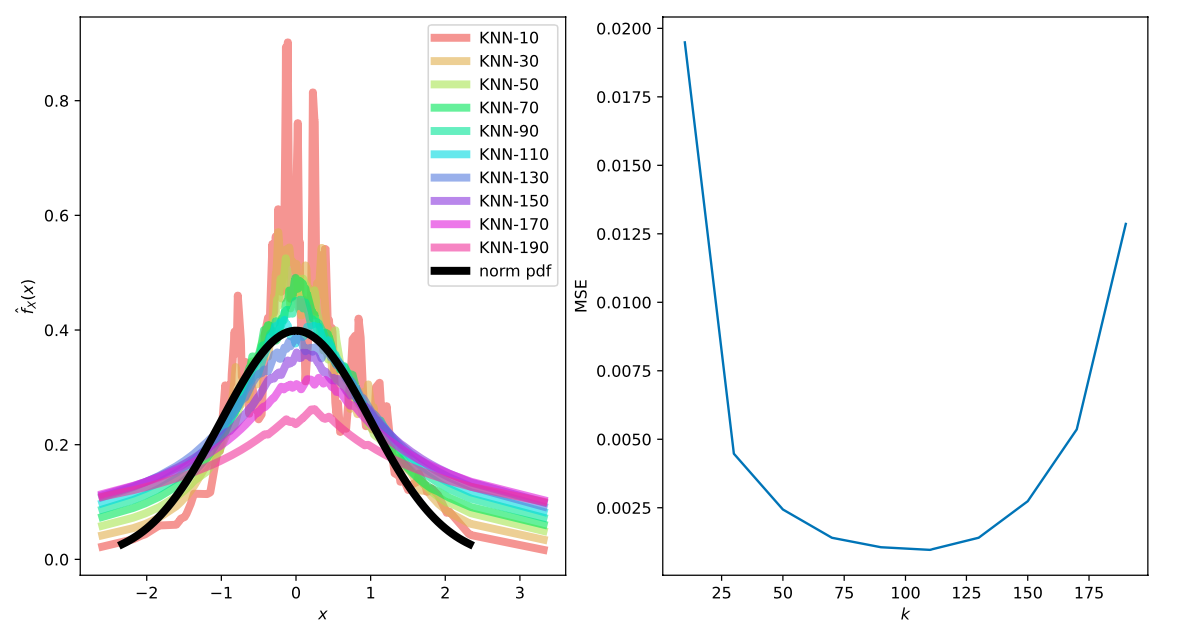
Now we can do a little experiment with a known true distribution in 1D.
import seaborn as sns
import matplotlib.pyplot as plt
from scipy.stats import norm
from sklearn.metrics import mean_squared_error as MSE

fig, ax = plt.subplots(1, 2)

# draw 200 samples from a 1D standard normal distribution
rv = norm()
r = np.array(norm.rvs(size=200))
r = r.reshape(-1, 1)

colors = sns.color_palette("hls", 10)
ks = []
mses = []

# test different values of k
for i,k in enumerate(range(10, 200, 20)):
    densities = knn_density(r, r, k=k)
    points = sorted(zip(r, densities), key=lambda x:x[0])
    x = [p[0] for p in points]
    y = [p[1] for p in points]
    ax[0].plot(x, y, '-', color=colors[i], lw=5, alpha=0.6, label=f'KNN-{k}')
    mse = MSE(y, norm.pdf(x))
    mses.append(mse)
    ks.append(k)

# plot the PDF of standard normal
x = np.linspace(norm.ppf(0.01),
               norm.ppf(0.99), 100)
ax[0].plot(x, norm.pdf(x),
           '-', color='black',
           lw=5, alpha=1, label='norm pdf')

ax[1].plot(ks, mses)
ax[1].set_xlabel("$k$")
ax[1].set_ylabel("MSE")

ax[0].set_xlabel("$x$")
ax[0].set_ylabel("$\hat{f}_{X}(x)$")
ax[0].legend()
plt.show()
We get the following plots for the density estimate at each sample (left) and the resulting mean squared error for different values of $k$ where you can clearly see the bias-variance tradeoff..